Python Worksheet
Setup
Import packages
import numpy as np
import pandas as pd
import matplotlib.pyplot as plt
import seaborn as sns
import statsmodels.api as sm
import statsmodels.formula.api as smf

# Remove unrelated warning
import warnings
warnings.simplefilter(action="ignore", category=FutureWarning)
/usr/local/lib/python3.7/dist-packages/statsmodels/tools/_testing.py:19: FutureWarning: pandas.util.testing is deprecated. Use the functions in the public API at pandas.testing instead.
  import pandas.util.testing as tm
Download OASIS Dataset
We’ll be downloading the data from http://www.oasis-brains.org/pdf/oasis_longitudinal.csv.
A full explanation of the data can be found in:
Open Access Series of Imaging Studies (OASIS): Longitudinal MRI Data in Nondemented and Demented Older Adults. Marcus, DS, Fotenos, AF, Csernansky, JG, Morris, JC, Buckner, RL, 2010. Journal of Cognitive Neuroscience, 22, 2677-2684. doi: 10.1162/jocn.2009.21407
df = pd.read_csv('http://www.oasis-brains.org/pdf/oasis_longitudinal.csv')
# Print out the top 5 rows of the DataFrame
df.head(5)
| Subject ID | MRI ID | Group | Visit | MR Delay | M/F | Hand | Age | EDUC | SES | MMSE | CDR | eTIV | nWBV | ASF | |
|---|---|---|---|---|---|---|---|---|---|---|---|---|---|---|---|
| 0 | OAS2_0001 | OAS2_0001_MR1 | Nondemented | 1 | 0 | M | R | 87 | 14 | 2.0 | 27.0 | 0.0 | 1987 | 0.696 | 0.883 |
| 1 | OAS2_0001 | OAS2_0001_MR2 | Nondemented | 2 | 457 | M | R | 88 | 14 | 2.0 | 30.0 | 0.0 | 2004 | 0.681 | 0.876 |
| 2 | OAS2_0002 | OAS2_0002_MR1 | Demented | 1 | 0 | M | R | 75 | 12 | NaN | 23.0 | 0.5 | 1678 | 0.736 | 1.046 |
| 3 | OAS2_0002 | OAS2_0002_MR2 | Demented | 2 | 560 | M | R | 76 | 12 | NaN | 28.0 | 0.5 | 1738 | 0.713 | 1.010 |
| 4 | OAS2_0002 | OAS2_0002_MR3 | Demented | 3 | 1895 | M | R | 80 | 12 | NaN | 22.0 | 0.5 | 1698 | 0.701 | 1.034 |
Pre-processing the Data
Dementia Status from CDR
We’re told in the associated paper (linked above) that the CDR values correspond to the following levels of severity:
0 = No dementia
0.5 = Very mild Dementia
1 = Mild Dementia
2 = Moderate Dementia
3 = Severe Dementia
So let’s derive this “Status” from the CDR values:
# Create a mapper from values to status/severity
cdr_mapper = {
    0: "No Dementia",
    0.5: "Very Mild Dementia",
    1: "Mild Dementia",
    2: "Moderate Dementia",
    3: "Severe Dementia",
}
# Create a column, mapping CDR values to this status
# Convert to categorical type, with severity as order
df["Status"] = pd.Categorical(
    df["CDR"].map(cdr_mapper),
    categories=cdr_mapper.values(),
    ordered=True
)
# Create colours for the different 'Status' categories
status_colours = {
    i:j for i,j in zip(cdr_mapper.values(), sns.color_palette("colorblind", 5))
}
Now we can look at this status, and how many records there are both overall, and at each of the visits (or time points).
# Let's look at how many records we have of each severity
df["Status"].value_counts()
No Dementia           206
Very Mild Dementia    123
Mild Dementia          41
Moderate Dementia       3
Severe Dementia         0
Name: Status, dtype: int64
# There are no records for "Severe Dementia", so we can tidy things up by removing this unused category
df["Status"] = df["Status"].cat.remove_unused_categories()
# How many of each status do we have at each visit?
df.groupby(["Visit", "Status"]).size()
Visit  Status
1      No Dementia           85
       Very Mild Dementia    52
       Mild Dementia         13
       Moderate Dementia      0
2      No Dementia           73
       Very Mild Dementia    49
       Mild Dementia         19
       Moderate Dementia      3
3      No Dementia           34
       Very Mild Dementia    18
       Mild Dementia          6
       Moderate Dementia      0
4      No Dementia           10
       Very Mild Dementia     3
       Mild Dementia          2
       Moderate Dementia      0
5      No Dementia            4
       Very Mild Dementia     1
       Mild Dementia          1
       Moderate Dementia      0
dtype: int64
Variable Types
df.dtypes
Subject ID      object
MRI ID          object
Group           object
Visit            int64
MR Delay         int64
M/F             object
Hand            object
Age              int64
EDUC             int64
SES            float64
MMSE           float64
CDR            float64
eTIV             int64
nWBV           float64
ASF            float64
Status        category
dtype: object
Note: Further coercing of types (e.g. “Visit” is ordinal) is good practice, but the necessity depends on your analysis.
Convert Categorical Data
df["Sex"] = df["M/F"].map({
  "M": 0,
  "F": 1
})
Visits & Baseline Data
df["Visit"].value_counts()
1    150
2    144
3     58
4     15
5      6
Name: Visit, dtype: int64
Filter for baseline data, and look at their status on arrival
df_baseline = df.loc[df["Visit"]==1]
df_baseline["Status"].value_counts()
No Dementia           85
Very Mild Dementia    52
Mild Dementia         13
Moderate Dementia      0
Name: Status, dtype: int64
Data Exploration & Analysis
Summarize Data
df.describe(include="all")
| Subject ID | MRI ID | Group | Visit | MR Delay | M/F | Hand | Age | EDUC | SES | MMSE | CDR | eTIV | nWBV | ASF | Status | Sex | |
|---|---|---|---|---|---|---|---|---|---|---|---|---|---|---|---|---|---|
| count | 373 | 373 | 373 | 373.000000 | 373.000000 | 373 | 373 | 373.000000 | 373.000000 | 354.000000 | 371.000000 | 373.000000 | 373.000000 | 373.000000 | 373.000000 | 373 | 373.000000 |
| unique | 150 | 373 | 3 | NaN | NaN | 2 | 1 | NaN | NaN | NaN | NaN | NaN | NaN | NaN | NaN | 4 | NaN |
| top | OAS2_0048 | OAS2_0179_MR2 | Nondemented | NaN | NaN | F | R | NaN | NaN | NaN | NaN | NaN | NaN | NaN | NaN | No Dementia | NaN |
| freq | 5 | 1 | 190 | NaN | NaN | 213 | 373 | NaN | NaN | NaN | NaN | NaN | NaN | NaN | NaN | 206 | NaN |
| mean | NaN | NaN | NaN | 1.882038 | 595.104558 | NaN | NaN | 77.013405 | 14.597855 | 2.460452 | 27.342318 | 0.290885 | 1488.128686 | 0.729568 | 1.195461 | NaN | 0.571046 |
| std | NaN | NaN | NaN | 0.922843 | 635.485118 | NaN | NaN | 7.640957 | 2.876339 | 1.134005 | 3.683244 | 0.374557 | 176.139286 | 0.037135 | 0.138092 | NaN | 0.495592 |
| min | NaN | NaN | NaN | 1.000000 | 0.000000 | NaN | NaN | 60.000000 | 6.000000 | 1.000000 | 4.000000 | 0.000000 | 1106.000000 | 0.644000 | 0.876000 | NaN | 0.000000 |
| 25% | NaN | NaN | NaN | 1.000000 | 0.000000 | NaN | NaN | 71.000000 | 12.000000 | 2.000000 | 27.000000 | 0.000000 | 1357.000000 | 0.700000 | 1.099000 | NaN | 0.000000 |
| 50% | NaN | NaN | NaN | 2.000000 | 552.000000 | NaN | NaN | 77.000000 | 15.000000 | 2.000000 | 29.000000 | 0.000000 | 1470.000000 | 0.729000 | 1.194000 | NaN | 1.000000 |
| 75% | NaN | NaN | NaN | 2.000000 | 873.000000 | NaN | NaN | 82.000000 | 16.000000 | 3.000000 | 30.000000 | 0.500000 | 1597.000000 | 0.756000 | 1.293000 | NaN | 1.000000 |
| max | NaN | NaN | NaN | 5.000000 | 2639.000000 | NaN | NaN | 98.000000 | 23.000000 | 5.000000 | 30.000000 | 2.000000 | 2004.000000 | 0.837000 | 1.587000 | NaN | 1.000000 |
Missing Data
# Count amount of missing data
df.isna().sum(0)
Subject ID     0
MRI ID         0
Group          0
Visit          0
MR Delay       0
M/F            0
Hand           0
Age            0
EDUC           0
SES           19
MMSE           2
CDR            0
eTIV           0
nWBV           0
ASF            0
Status         0
Sex            0
dtype: int64
Visualize Data
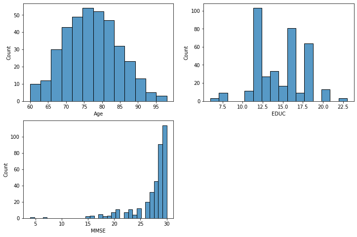
# Histograms
fig, axes = plt.subplots(2, 2, figsize=(12,8))

axes = axes.flatten()

for i, x_col in enumerate(["Age", "EDUC", "MMSE"]):
  sns.histplot(data=df, x=x_col, ax=axes[i])

fig.delaxes(axes[-1])
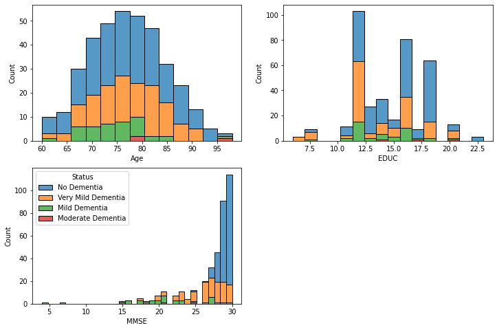
# Histograms stratified by dementia status
fig, axes = plt.subplots(2, 2, figsize=(12,8))
# Make it easier to loop over
axes = axes.flatten()
# Loop through the columns we want to plot a histogram for
for i, x_col in enumerate(["Age", "EDUC", "MMSE"]):
    sns.histplot(data=df, x=x_col, hue="Status", multiple="stack", ax=axes[i])
# Manually tidy up the legends
axes[0].get_legend().remove()
axes[1].get_legend().remove()
# Delete the extra axis (as we only plot 3 columns)
fig.delaxes(axes[-1])
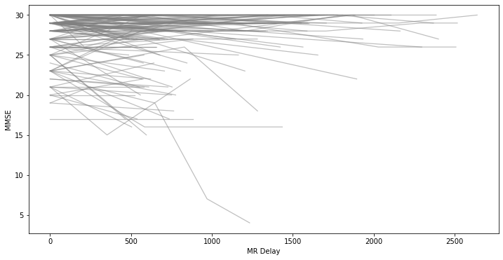
MMSE trajectories over time
We can visualize the MMSE trajectories of each subject over time to get an overall view of the cohort.
fig, ax = plt.subplots(figsize=(12,6))
for _, indiv_data in df.groupby("Subject ID"):
    ax = sns.lineplot(
        data=indiv_data,
        x="MR Delay",
        y="MMSE",
        ax=ax,
        color="grey",
        alpha=0.5,
        linewidth=1.25,
        linestyle="solid"
    )
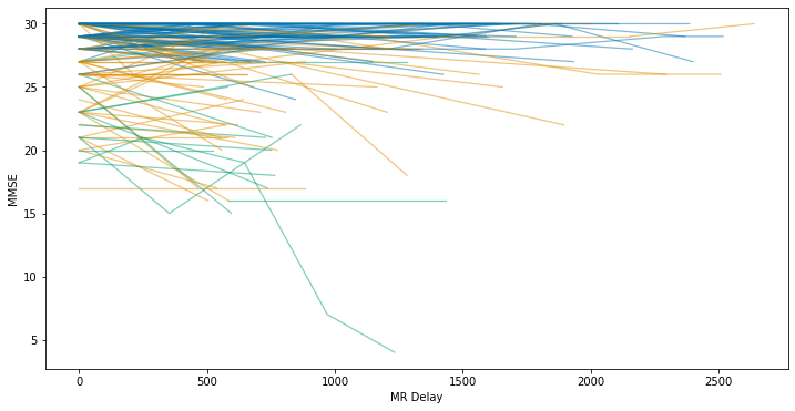
We can make this graph a little more interesting by adding colour to each line, corresponding to the dementia status:
fig, ax = plt.subplots(figsize=(12,6))

# Loop over the individual subjects
for group, indiv_data in df.groupby(["Subject ID"]):
    # Extract xy data
    xy = indiv_data[["MR Delay", "MMSE"]].values
    # Plot normally for patients that do not change status
    if len(indiv_data["Status"].unique()) == 1:
      ax.plot(
          xy[:, 0],
          xy[:, 1],
          color=status_colours[indiv_data["Status"].unique()[0]],
          alpha=0.5,
          linewidth=1.25
      )
    else:
      # Duplicate points to construct line segments of different colours
      for i, (start, stop) in enumerate(zip(xy[:-1], xy[1:])):
        x, y = zip(start, stop)
        ax.plot(
            x, y,
            color=status_colours[indiv_data["Status"].iloc[i]],
            alpha=0.5,
            linewidth=1.25
        )
# Add the labels
ax.set_xlabel("MR Delay")
ax.set_ylabel("MMSE")
Text(0, 0.5, 'MMSE')
Regression Analysis
Simple Linear Regression
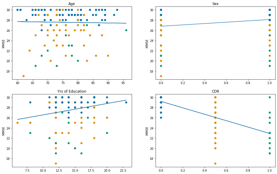
# Select the columns to iterate over
x_cols = ["Age", "Sex", "EDUC", "CDR"]
# Choose nicer names to display for each column
x_labels = ["Age", "Sex", "Yrs of Education", "CDR"]

fig, axes = plt.subplots(2,2, figsize=(16,10))

# Select the dependent variable
y = df_baseline["MMSE"].values
# Loop over the columns to fit each regression
for x_col, label, ax in zip(x_cols, x_labels, axes.flatten()):
    # Select x data
    x = df_baseline[x_col].values
    # Create the model
    model = sm.OLS(
        y, sm.add_constant(x)
    )
    # Fit the model
    res = model.fit()
    # Add a plot with regression line
    ax.plot(x, res.predict())
    # and the raw data
    ax.scatter(x, y, c=[status_colours[i] for i in df_baseline["Status"]])
    ax.set_title(label)
    ax.set_ylabel("MMSE")
    # Print the R^2
    print(f"{label} vs MMSE: R-squared = {res.rsquared:.3f}")
Age vs MMSE: R-squared = 0.001
Sex vs MMSE: R-squared = 0.048
Yrs of Education vs MMSE: R-squared = 0.047
CDR vs MMSE: R-squared = 0.479
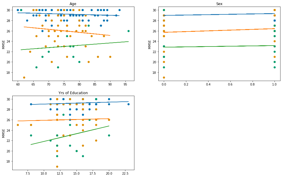
Then we can do the same again, but this time stratify by the dementia status (not including CDR this time):
x_cols = ["Age", "Sex", "EDUC"]
x_labels = ["Age", "Sex", "Yrs of Education"]

fig, axes = plt.subplots(2,2, figsize=(16,10))
axes = axes.flatten()

for x_col, label, ax in zip(x_cols, x_labels, axes):
    for name, group_data in df_baseline.groupby("Status", observed=True):
        y = group_data["MMSE"]
        x = group_data[x_col]
        model = sm.OLS(
            y, sm.add_constant(x)
        )
        res = model.fit()

        ax.plot(x, res.predict())
        ax.scatter(x, y, color=status_colours[name])
    ax.set_title(label)
    ax.set_ylabel("MMSE")
# Delete the extra axis (as we only plot 3 columns)
fig.delaxes(axes[-1])
Multiple Linear Regression
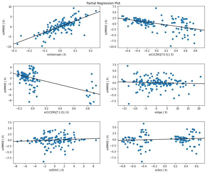
We can create a regression model using age, sex, education, and CDR as our independent variables together:
# Create string for our independent variables
x = "Age + EDUC + Sex + C(CDR)"
# And select the dependent one
y = "MMSE"

mod = smf.ols(formula = f"{y} ~ {x}", data=df_baseline)
res = mod.fit()

# Print out a nice summary of results
print(res.summary())
                            OLS Regression Results
==============================================================================
Dep. Variable:                   MMSE   R-squared:                       0.493
Model:                            OLS   Adj. R-squared:                  0.475
Method:                 Least Squares   F-statistic:                     27.95
Date:                Thu, 08 Jul 2021   Prob (F-statistic):           1.02e-19
Time:                        10:03:10   Log-Likelihood:                -324.67
No. Observations:                 150   AIC:                             661.3
Df Residuals:                     144   BIC:                             679.4
Df Model:                           5
Covariance Type:            nonrobust
=================================================================================
                    coef    std err          t      P>|t|      [0.025      0.975]
---------------------------------------------------------------------------------
Intercept        29.1743      2.140     13.632      0.000      24.944      33.404
C(CDR)[T.0.5]    -2.9600      0.411     -7.209      0.000      -3.772      -2.148
C(CDR)[T.1.0]    -6.0383      0.649     -9.305      0.000      -7.321      -4.756
Age              -0.0194      0.024     -0.825      0.411      -0.066       0.027
EDUC              0.0734      0.065      1.137      0.257      -0.054       0.201
Sex               0.5643      0.374      1.511      0.133      -0.174       1.303
==============================================================================
Omnibus:                       23.128   Durbin-Watson:                   1.929
Prob(Omnibus):                  0.000   Jarque-Bera (JB):               53.918
Skew:                          -0.623   Prob(JB):                     1.96e-12
Kurtosis:                       5.660   Cond. No.                         943.
==============================================================================

Warnings:
[1] Standard Errors assume that the covariance matrix of the errors is correctly specified.
# Call statsmodel function for partial regression plot
fig = sm.graphics.plot_partregress_grid(res)
# Making the output nicer
fig.set_figheight(10)
fig.set_figwidth(12)
fig.tight_layout(pad=3)
Results Table
Either using some of the analysis above, or through additional analysis of your own, create a summary results table below. What it includes is up to you, the overall aim is to get familiar with creating tables in markdown.
Export to PDF
Now we can export this report to PDF, using the steps below.
Note: You may need to change the paths and filenames depending your Google Drive structure, and what you have named this notebook.
# Install what we need to create the PDF
%%capture
!apt update
!apt install texlive-xetex texlive-fonts-recommended texlive-generic-recommended
# Mount Google Drive
from google.colab import drive
drive.mount('/content/gdrive')
Drive already mounted at /content/gdrive; to attempt to forcibly remount, call drive.mount("/content/gdrive", force_remount=True).
# Create a DEMON folder and move this notebook into it
%%bash
mkdir -p gdrive/MyDrive/DEMON/
if [ -f gdrive/MyDrive/Reproducible_Reporting.ipynb ]; then
  mv gdrive/MyDrive/Reproducible_Reporting.ipynb gdrive/MyDrive/DEMON/Reproducible_Reporting.ipynb
fi
ls gdrive/MyDrive/DEMON/
Reproducible_Reporting.ipynb
# Change to the drive we created above
%cd gdrive/MyDrive/DEMON/
/content/gdrive/MyDrive/DEMON
!jupyter nbconvert Reproducible_Reporting.ipynb --to pdf --output ./Reproducible_Reporting.pdf
[NbConvertApp] Converting notebook Reproducible_Reporting.ipynb to pdf
[NbConvertApp] Writing 49953 bytes to ./notebook.tex
[NbConvertApp] Building PDF
[NbConvertApp] Running xelatex 3 times: [u'xelatex', u'./notebook.tex', '-quiet']
[NbConvertApp] Running bibtex 1 time: [u'bibtex', u'./notebook']
[NbConvertApp] WARNING | bibtex had problems, most likely because there were no citations
[NbConvertApp] PDF successfully created
[NbConvertApp] Writing 59264 bytes to ./Reproducible_Reporting.pdf